Mathematics often feels most useful when it stops looking like schoolwork and starts acting like infrastructure. Integrals do exactly that. In engineering and computing, they help turn raw variation into something measurable, predictable, and usable.
A filtered audio track, a believable shadow in a game engine, or a probabilistic model that can cope with uncertainty often depends on the same core move: add up many tiny contributions across time, space, frequency, or probability.
For many readers, the surprising part is not that integrals appear in advanced technical work. The surprising part is how often the same mathematical idea reappears in very different jobs.
Signal processing uses integrals to combine an input with a system response and to move between time and frequency descriptions. Computer graphics uses integrals to estimate how much light reaches a camera through a pixel.
Data modeling uses integrals to compute expectations, marginal probabilities, and parameter estimates when direct answers are messy or impossible.
Highlights
Why Integrals Show Up So Often
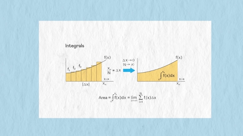
An integral is a controlled way to accumulate small pieces into one result. In a classroom, that idea often appears as “area under a curve.” In applied work, the phrase is too narrow.
Readers who want to revisit integral calculus from a more structured teaching angle can also explore Qui Si Risolve alongside articles like this one.
A signal engineer may integrate over time. A graphics engineer may integrate light over directions or pixel area. A data scientist may integrate a probability density over possible parameter values. Same logic, different setting.
A compact way to think about the role of an integral is given below.
| Field | What Gets Accumulated | Why It Matters |
| Signal processing | Signal contributions over time or frequency | Filtering, system response, spectrum analysis |
| Computer graphics | Radiance or sample contributions over paths, angles, or pixel area | Realistic shading, anti-aliasing, global illumination |
| Data modeling | Probability density, expected loss, or model error | Inference, forecasting, uncertainty handling, fitting |
Across all three fields, an integral answers a practical question: if countless tiny influences matter, how do you combine them without losing the structure of the problem?
Integrals in Signal Processing
Signal processing offers one of the clearest examples because the math maps closely to familiar experiences such as music, speech, radio, and medical sensing.
Convolution: How Systems Respond to Inputs
A classic result from signals and systems says that for a linear time-invariant system, the output can be written as a convolution of the input with the system’s impulse response.
MIT course material writes that relationship as an integral of the input multiplied by a shifted response function. In plain language, every instant of the input leaves a small trace, and the total output is the sum of all those traces.
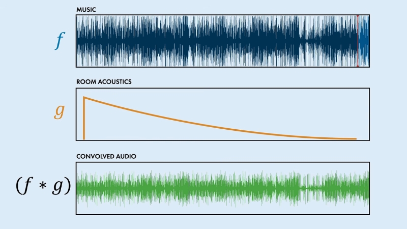
That idea is easier to picture with sound. Imagine a short clap inside a cathedral. The clap happens once, but the room produces echoes and decay over time.
Now imagine a singer performing in the same space. Each tiny slice of the voice interacts with the room in a similar way. Convolution adds up all those delayed and weighted echoes to produce the sound heard by a microphone.
Common uses include:
A moving average filter, for example, can be viewed as an integral or sum that blends nearby values. A low-pass filter works on the same principle, reducing rapid fluctuations while preserving slower variation.
Engineers use that move to remove high-frequency noise from ECG signals, stabilize industrial measurements, or make speech easier to process.
Fourier Transform: Reading a Signal by Frequency
Another central tool is the Fourier transform. MIT notes define the continuous Fourier transform as an integral that multiplies a signal by a complex exponential and sums the result over all time.
Operationally, that converts a time-based signal into a frequency-based description. Why does that matter? Because many real-world questions are easier in frequency language than in time language.
A few examples:
Suppose a machine motor begins to fail. A time-domain waveform may look messy. A frequency-domain view can reveal a sharp spike at a particular vibration frequency tied to misalignment, bearing wear, or imbalance. Same data, better lens.
Fourier analysis also explains why filters work. A signal with slow variation and sudden spikes contains different frequency content. Once a signal is expressed in the frequency domain, suppressing unwanted ranges becomes more direct.
MIT graphics notes on sampling even stress a related fact: convolution in one domain corresponds to multiplication in the other, which is one reason frequency-domain analysis is so powerful across engineering and graphics work.
Continuous Models Still Matter in a Digital World
Modern devices are digital, so a fair question comes up: why keep talking about integrals when computers often use sums?
Because the underlying phenomena are often continuous before sampling. Sound waves, light, voltage, motion, and temperature do not arrive in neatly packaged integers.
Engineers frequently begin with continuous models, use integrals to describe behavior, then approximate numerically after sampling.
MIT graphics lectures make a similar point about images: sampling and reconstruction start from an underlying continuous signal, then practical filters approximate the needed operations.
That bridge between continuous math and discrete computation is a recurring pattern in applied science. The integral gives the ideal formulation. Numerical methods give the computable version.
Integrals in Computer Graphics
Graphics may look far removed from classical calculus, but some of the most important problems in rendering are integral problems at heart.
The Rendering Equation and Light Transport
Physically based rendering grew around a crucial insight from Jim Kajiya’s work in the 1980s.
PBRT, a standard reference in rendering, describes that contribution as a rigorous formulation of rendering as a light transport integral equation, along with Monte Carlo integration methods for solving it.
What does that mean in ordinary language?
When a camera looks at a scene, the color recorded at one point depends on more than a single light ray. Light can bounce off walls, scatter through fog, reflect from glossy paint, pass through glass, and lose energy along the way.
A realistic image needs to account for many possible incoming directions and interactions. An integral is the natural tool because image formation depends on accumulating many tiny light contributions.
In film rendering, game engines, and architectural visualization, that principle appears in jobs such as:
When a rendered room looks believable, part of the reason is that the software has estimated how light from many paths contributes to each visible point.
Monte Carlo Integration: Why Graphics Uses Randomness
Some rendering integrals are too large or too high-dimensional for neat closed-form solutions. PBRT explains why Monte Carlo integration became a key method: randomness can estimate important rendering integrals with a convergence rate that does not depend on the dimensionality of the integrand.
In practice, that is why renderers fire many sample rays instead of trying to solve every light interaction exactly.
A rough sketch of the logic works as follows:
- Pick sample paths or directions according to a probability rule.
- Evaluate how much light each sample contributes.
- Average the results.
- Use more samples to reduce visible noise.
Anyone who has watched a path-traced image start grainy and gradually clean up has seen numerical integration in action.
Graphics programmers often make tradeoffs here. More samples usually mean less noise and more accurate lighting, but also more computation.
Real-time graphics has to balance image quality against frame rate. Offline film rendering can afford heavier sampling.
Anti-Aliasing, Texture Filtering, and Pixel Footprints
Integrals also appear in a quieter but extremely important part of graphics: sampling and filtering. MIT graphics lecture material notes that aliasing appears when a signal is sampled and reconstructed poorly, and that filters act as weighting functions or convolution kernels.
The same notes explain that spatial filtering can be viewed as computing an integration over the extent of a pixel, equivalent to convolving the texture with a filter kernel.
That statement has huge practical consequences.
A pixel is not magically immune to detail finer than its size. If a scene contains very thin lines, checkerboard textures, or distant repeating patterns, naive point sampling can produce shimmer, moiré patterns, and jagged edges.
Integrating color over the pixel footprint gives a better estimate of what the pixel should display.
A simple comparison helps:
| Graphics Problem | Naive Approach | Integral-Based Idea |
| Edge rendering | Sample one point per pixel | Average coverage over pixel area |
| Texture minification | Read one texel | Filter over a region in texture space |
| Global illumination | Follow one idealized path | Accumulate many path contributions |
Mipmapping, supersampling, bilinear filtering, bicubic filtering, and Gaussian filtering all live in that broader family of approximation methods.
Exact integration is often too expensive, so graphics systems use prefiltered textures or sample-based estimates that are good enough for the target workload.
Volume Rendering and Transmittance
Another useful case comes from fog, smoke, clouds, and medical volume visualization. PBRT’s treatment of transmittance notes that graphics often estimate optical thickness through sums, yet also works from equations designed to enable unbiased estimation.
Under the hood, the renderer is accounting for how much light is absorbed or scattered as it travels through a medium.
For a non-specialist, a good mental picture is sunlight moving through mist. Color at the camera depends on how much light survives the trip and how much new scattered light joins along the path. Again, an accumulation problem. Again, an integral.
Integrals in Data Modeling
Data modeling is a broad label, so the role of integrals depends on the kind of model involved. In practice, three jobs appear again and again: computing expectations, handling uncertainty, and fitting models to observations.
Expectations: Turning Distributions Into Useful Numbers
NIST material on probability and uncertainty defines the expectation of a function of a random variable, for the continuous case, as an integral of the function times the probability density.
That idea sits at the center of statistical work because a model rarely stops at “what values are possible?” A working model has to answer questions like average cost, expected wait time, average lifetime, or expected prediction error.
A few concrete examples:
If a bulb’s lifetime follows a continuous distribution, probability over an interval comes from integrating the density over that interval.
NIST material also shows that the mean of an exponential lifetime model can be computed from the defining density.
For working analysts, that is the difference between a descriptive curve and a usable business or engineering forecast.
Marginalization: Integrating Out What You Do Not Observe
Data is often incomplete. Some variables are missing, latent, or treated as nuisance parameters. Bayesian statistics handles that problem by integrating over unknowns rather than pretending they do not exist.
Stanford notes on Bayesian analysis show the continuous marginal distribution as an integral over a joint density.
A practical example helps.
Imagine a medical model predicting disease risk from symptoms and lab values, while some biological factor remains unobserved.
One route would be to guess a single value for the hidden factor and move on. A more principled route is to average over plausible values weighted by probability. An integral performs that averaging.
Same pattern appears in:
Why analysts care so much about that step is simple. Integrating over uncertainty often produces predictions that are more stable and more honest about what the model does and does not know.
Least Squares, Continuous Error, and Model Fitting
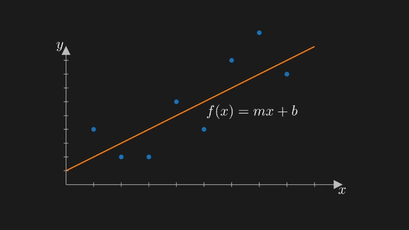
MIT material on fitting models to data describes least squares as a common way to connect models and measurements through minimization of misfit.
In many settings, especially when models are continuous in time or space, the error being minimized can be written as an integral of squared differences.
That matters in areas such as:
Suppose a researcher has temperature data collected over time and a differential-equation model for heat flow. One way to estimate unknown parameters is to choose values that make the model curve stay close to the measurements.
If closeness is measured over a whole interval rather than only at a few points, an integral gives the natural error measure.
Many machine learning methods use discrete sums because data arrives in rows. Even so, the underlying theory often leans on continuous objectives, expected risk, or probability densities.
In other words, a great deal of modern modeling still carries calculus in the frame, even when code uses batches and matrices.
Why Numerical Integration Matters in Modern Modeling
Closed-form integrals are pleasant when available, but much of modern modeling does not offer that luxury. Posterior distributions, expected utility, and marginal likelihood can become hard to compute fast.
NIST discusses Markov chain Monte Carlo as a route for obtaining samples from posterior distributions when closed forms are unavailable. In applied terms, one often estimates an integral by simulation rather than solving it symbolically.
That approach shows up across science and industry:
A large share of “advanced modeling” is really careful numerical integration wearing modern software clothes.
Shared Patterns Across the Three Fields
View this post on Instagram
Signal processing, graphics, and data modeling use different languages, but the same mathematical habits keep showing up.
1. Small Contributions Add Up
In signal processing, each shifted piece of an input contributes to the output. In graphics, each light path or sample contributes to a pixel value. In statistics, each part of a density contributes to a probability or expectation.
2. Exact Formulas Often Give Way to Approximation
Very few production systems rely on pen-and-paper integration alone. Engineers sample, approximate, prefilter, or simulate. Renderers use Monte Carlo estimates. Signal systems use discretization and fast transforms. Statistical workflows use quadrature, optimization, or MCMC.
3. Good Results Depend on the Right Domain
A signal may be easier to analyze in frequency space. A graphics problem may be easier to treat over pixel area or path space. A statistical problem may become manageable after moving from raw observations to densities and expectations. Integrals help formalize that change of viewpoint.
Final Thoughts
@mathscribbles Replying to @itsrobbietime let’s give it a shot! #mathematics #calculus #ilovemath #integral #mathtok ♬ Saturday – wizzow
Integrals earn their place in modern computing because many technical problems are accumulation problems.
Signal processing adds up the influence of past input and frequency content. Graphics adds up light over space, direction, and path. Data modeling adds up probability, loss, and uncertainty across possibilities.
Different industries, different software stacks, same mathematical backbone.
Anyone trying to read modern engineering or data work more clearly will benefit from seeing integrals in that practical light.
They are less about textbook ritual and more about a reliable way to combine many small effects into one decision, image, forecast, or signal.